Logistic regression can fail with sum of squares¶

import numpy as np
import pandas as pd
import matplotlib.pyplot as plt
from scipy.optimize import minimize

We read in the mtcars dataset that will be very familiar to users of R:

mtcars = pd.read_csv('mtcars.csv')
mtcars.head()

	mpg	cyl	disp	hp	drat	wt	qsec	vs	am	gear	carb
0	21.0	6	160.0	110	3.90	2.620	16.46	0	1	4	4
1	21.0	6	160.0	110	3.90	2.875	17.02	0	1	4	4
2	22.8	4	108.0	93	3.85	2.320	18.61	1	1	4	1
3	21.4	6	258.0	110	3.08	3.215	19.44	1	0	3	1
4	18.7	8	360.0	175	3.15	3.440	17.02	0	0	3	2

This dataset has one row per make and model of car. The columns have various measures and other information about each make and model.

The columns we are interested in here are:

mpg: Miles/(US) gallon
am: Transmission (0 = automatic, 1 = manual)

Notice that am is already numeric, and so is already a dummy variable.

mpg = mtcars['mpg']
am_dummy = mtcars['am']

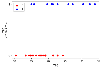
We will try to predict whether the car has an automatic transmission (column am) using the miles per gallon measure (column mpg).

Here is a plot of the am values against the mpg values:

# Code to make nice plots for binary columns.  Please ignore.
def plot_binary(df, x_name, bin_name, bin_labels=(0, 1),
                color_names=('red', 'blue')):
    x_vals = df[x_name]
    bin_vals = df[bin_name]
    # Build plot, add custom label.
    dummy = bin_vals.replace(bin_labels, (0, 1))
    colors = bin_vals.replace(bin_labels, color_names)
    plt.scatter(x_vals, dummy, c=colors)
    plt.xlabel(x_name)
    plt.ylabel('%s\n0 = %s, 1 = %s' % (x_name, bin_labels[0], bin_labels[1]))
    plt.yticks([0, 1]);  # Just label 0 and 1 on the y axis.
    # Put a custom legend on the plot.  This code is a little obscure.
    plt.scatter([], [], c=color_names[0], label=bin_labels[0])
    plt.scatter([], [], c=color_names[1], label=bin_labels[1])

plot_binary(mtcars, 'mpg', 'am')
plt.legend();

We need our machinery for calculating the inverse logit transformation, converting from the log-odds-ratio straight line prediction to the sigmoid prediction.

def inv_logit(y):
    """ Reverse logit transformation
    """
    odds_ratios = np.exp(y)  # Reverse the log operation.
    return odds_ratios / (odds_ratios + 1)  # Reverse odds ratios operation.


def params2pps(intercept, slope, x):
    """ Calculate predicted probabilities of 1 for each observation.
    """
    # Predicted log odds of being in class 1.
    predicted_log_odds = intercept + slope * x
    return inv_logit(predicted_log_odds)

This is our simple root mean square cost function comparing the sigmoid p predictions to the 0 / 1 labels

def ss_logit(c_s, x_values, y_values):
    # Unpack intercept and slope into values.
    intercept, slope = c_s
    # Predicted p values on sigmoid
    pps = params2pps(intercept, slope, x_values)
    # Prediction errors.
    sigmoid_error = y_values - pps
    # Sum of squared error
    return np.sum(sigmoid_error ** 2)

We run minimize using some (it turns out) close-enough initial values for the log-odds intercept and slope:

# Guessed log-odds intercept slope of -5, 0.5
mr_ss_ok = minimize(ss_logit, [-5, 0.5], args=(mpg, am_dummy))
mr_ss_ok

/Users/Olsonac-admin/opt/anaconda3/lib/python3.8/site-packages/pandas/core/arraylike.py:364: RuntimeWarning: overflow encountered in exp
  result = getattr(ufunc, method)(*inputs, **kwargs)

      fun: 4.903124915254921
 hess_inv: array([[19.31261058, -0.91067068],
       [-0.91067068,  0.04409889]])
      jac: array([-1.19209290e-07, -2.20537186e-06])
  message: 'Optimization terminated successfully.'
     nfev: 120
      nit: 10
     njev: 40
   status: 0
  success: True
        x: array([-6.164422  ,  0.28186366])

The prediction sigmoid looks reasonable:

inter_ok, slope_ok = mr_ss_ok.x
predicted_ok = inv_logit(inter_ok + slope_ok * mpg)

plot_binary(mtcars, 'mpg', 'am')
plt.scatter(mpg, predicted_ok, c='gold', label='SS fit, OK start')
plt.legend();

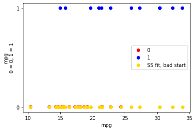
But - if we start with a not-so-close initial guess for the intercept and slope, minimize gets terribly lost:

# Guessed log-odds intercept slope of 1, 1
mr_ss_not_ok = minimize(ss_logit, [1, 1], args=(mpg, am_dummy))
mr_ss_not_ok

      fun: 12.99999999997786
 hess_inv: array([[1, 0],
       [0, 1]])
      jac: array([0., 0.])
  message: 'Optimization terminated successfully.'
     nfev: 24
      nit: 1
     njev: 8
   status: 0
  success: True
        x: array([ 0.74090123, -1.74592614])

The prediction sigmoid fails completely:

inter_not_ok, slope_not_ok = mr_ss_not_ok.x
predicted_not_ok = inv_logit(inter_not_ok + slope_not_ok * mpg)

plot_binary(mtcars, 'mpg', 'am')
plt.scatter(mpg, predicted_not_ok, c='gold', label='SS fit, bad start')
plt.legend();

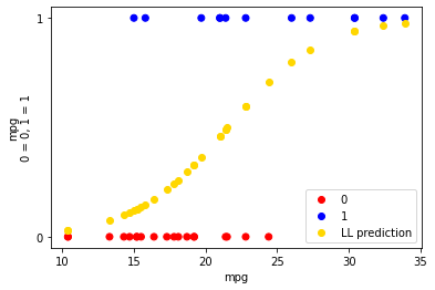
Can we do better with the maximum likelihood estimate (MLE) cost function?

def logit_reg_cost(intercept_and_slope, x, y):
    """ Cost function for maximum likelihood
    """
    intercept, slope = intercept_and_slope
    pp1 = params2pps(intercept, slope, x)
    p_of_y = y * pp1 + (1 - y) * (1 - pp1)
    log_likelihood = np.sum(np.log(p_of_y))
    return -log_likelihood

Here we pass some absolutely terrible initial guesses for the intercept and slope:

mr_LL = minimize(logit_reg_cost, [10, -5], args=(mpg, am_dummy))
mr_LL

      fun: 14.8375838241203
 hess_inv: array([[ 5.57233541, -0.26759306],
       [-0.26759306,  0.01337518]])
      jac: array([-1.19209290e-07, -4.17232513e-06])
  message: 'Optimization terminated successfully.'
     nfev: 57
      nit: 13
     njev: 19
   status: 0
  success: True
        x: array([-6.60352228,  0.30702797])

The fit is still reasonable:

inter_LL, slope_LL = mr_LL.x
predicted_LL = inv_logit(inter_LL + slope_LL * mpg)

plot_binary(mtcars, 'mpg', 'am')
plt.scatter(mpg, predicted_LL, c='gold', label='LL prediction')
plt.legend();

As we have seen before, the MLE fit above is the same algorithm that Statmodels and other packages use.

import statsmodels.formula.api as smf

model = smf.logit('am ~ mpg', data=mtcars)
fit = model.fit()
fit.summary()

Optimization terminated successfully.
         Current function value: 0.463674
         Iterations 6

Logit Regression Results
Dep. Variable:	am	No. Observations:	32
Model:	Logit	Df Residuals:	30
Method:	MLE	Df Model:	1
Date:	Tue, 30 Nov 2021	Pseudo R-squ.:	0.3135
Time:	22:06:03	Log-Likelihood:	-14.838
converged:	True	LL-Null:	-21.615
Covariance Type:	nonrobust	LLR p-value:	0.0002317

	coef	std err	z	P>\|z\|	[0.025	0.975]
Intercept	-6.6035	2.351	-2.808	0.005	-11.212	-1.995
mpg	0.3070	0.115	2.673	0.008	0.082	0.532

Notice that the intercept and slope coefficients are the same as the ones we found with the MLE cost function and minimize.

Coding for Data - 2021 edition

Logistic regression can fail with sum of squares¶